Proof: Attention Values Correlate After Layer 1

And what it means for the L1 vs L2 normalization debate.

Thesis: Depth two attention generically makes the layer-2 values cross-token correlated. Conditional on fixed attention weights (or in a fixed-weights surrogate), variance along any fixed unit direction must use the quadratic form shown below rather than the norm-only identity.

\(\mathrm{Var}(u^\top S \mid A) = A^\top \Sigma_u A.\)

Variance analyses of attention often begin with a convenient simplification:

If the per position value vectors are uncorrelated and isotropic with covariance

\(\mathrm{Cov}(V_j) = \sigma^2 I,\)

then for a fixed attention weight vector A the output

\(S = \sum_{j=1}^N A_j V_j\)

satisfies

\(\mathrm{Var}(u^\top S) = \sigma^2\|A\|_2^2\)

for any fixed unit direction u.

That identity is correct in that special case. But it’s not a property that survives depth.

The post makes one structural claim and separates it from magnitude and empirics:

1. Structural theorem: In a depth 2 transformer, the layer 2 values are generically cross-token correlated, even if the input tokens start independent. Layer 1 can already correlate outputs via overlapping attention weights; the new claim is that the values fed into layer 2 are no longer cross-token independent.

2. Implication for normalization arguments: Once values are correlated, the correct variance along any fixed direction, conditional on weights, is given by the quadratic form above. The norm-only identity is a special case. Whether the “extra terms” are practically large is an empirical question, one you can diagnose with a single statistic measuring common mode covariance.

This result is related to rank collapse phenomena studied in the signal propagation literature, where token representations become increasingly correlated at depth. See References for Noci et al. 2022 and Cowsik et al. 2024. The contribution here is to connect that structural fact directly to the norm-squared variance identity used in normalization arguments.

I distinguish two mechanisms that create cross token correlation and label the assumptions where they are used.

---

1) Setup and notation

Let X₁, …, Xₙ be i.i.d. d-dimensional tokens with zero mean and nondegenerate covariance. Assume enough moments so that covariances are finite (e.g., subgaussian or bounded support inputs).

Consider a single head self attention layer:

\(q_i = W_Q X_i,\quad k_j = W_K X_j,\quad v_j = W_V X_j,\)

\(a_{ij} = \frac{\exp(\langle q_i,k_j\rangle/\sqrt{d_k})}{\sum_{t=1}^N \exp(\langle q_i,k_t\rangle/\sqrt{d_k})}.\)

Assume full support: each visible attention weight is strictly positive (ordinary softmax over a finite set satisfies this; for causal masks, this holds within the visible prefix).

The attention output at token i is

\(H_i = \sum_{j=1}^N a_{ij} v_j.\)

A two layer attention only stack forms layer 2 values by

\(V_i^{(2)} = W_V^{(2)} H_i,\)

and layer 2 then attends over the set of layer 2 values.

(Residual, norm, and MLP are discussed later; that discussion is informal and focuses on the attention update itself.)

---

2) Two mechanisms for cross token correlation (don’t conflate them)

It’s easy to accidentally mix two different sources of correlation:

Mechanism A: values become correlated across positions (depth effect)

At depth two or more, the values going into layer 2 are functions of overlapping mixtures of the original tokens, so the cross-token covariance matrix across positions is typically nondiagonal. The main theorem below proves this mechanism.

Mechanism B: even i.i.d. values can yield correlated outputs (overlapping weights)

Even if values at each position were independent, two different queries can produce outputs that are correlated if their attention weights overlap.

This mechanism is often summarized by a “cosine similarity of attention rows” identity, but that identity must be read as conditional on the weights (or under a model where weights are independent of values).

A clean way to keep both mechanisms straight is the law of total covariance. Fix a scalar direction u and define

\(Y_j = u^\top V_j,\)

and let

\(S_i = \sum_{j=1}^N A_{ij} Y_j,\qquad S_\ell = \sum_{j=1}^N A_{\ell j} Y_j,\)

where the A(i,j) are the (random) attention weights depending on the same input as the values.

Then

\(\mathrm{Cov}(S_i,S_\ell) = \mathbb{E}\left[\mathrm{Cov}(S_i,S_\ell\mid A)\right] + \mathrm{Cov}\left(\mathbb{E}[S_i\mid A],\ \mathbb{E}[S_\ell\mid A]\right).\)

• The first term is the mixing through covariance term. Conditional on A,

  \(\mathrm{Cov}(S_i,S_\ell \mid A) = A_i^\top \Sigma_{Y\mid A} A_\ell,\)

  
  where the weight vectors for positions i and ℓ appear, and the conditional covariance of Y given A appears in the middle. Note: even if the scalar values are independent marginally, conditioning on A generally induces dependence among them, so the conditional covariance need not be diagonal. If A is independent of Y and the conditional covariance is constant, this reduces to the fixed-weights quadratic form

  \(A_i^\top \Sigma_Y A_\ell.\)

• The second term captures additional dependence coming from the fact that weights depend on data and can correlate with the values.

The main theorem addresses Mechanism A, showing the cross-token covariance becomes nondiagonal at depth 2.

---

3) Main theorem: depth 2 induces cross token covariance in layer 2 values

Theorem (Depth 2 breaks cross-token independence of layer-2 values)

For any distinct positions i and ℓ, under the assumptions in Section 1 and for generic (nondegenerate) parameters in a two-layer attention-only stack,

\(\mathrm{Cov}\big(V_i^{(2)},V_\ell^{(2)}\big) \neq 0,\)

where the layer-2 values are defined by

\(V_i^{(2)} = W_V^{(2)} H_i,\)

even though the inputs are independent. Layer 1 can already produce correlated outputs through overlapping weights (Mechanism B); the new point is that by depth 2 the values themselves are no longer cross-token independent. In particular, the simplifying assumption “values are uncorrelated across tokens” is not depth-stable.

If some scalar projection of the layer-2 values has nonzero cross-token covariance, then the matrix covariance is nonzero, so scalar projections are enough to witness the claim. At the uniform attention witness the cross covariance is symmetric, so a nonzero matrix implies some nonzero quadratic form.

“Generic” here means: the set of parameters for which this covariance is exactly zero is not structurally enforced and occupies a measure zero (or otherwise nongeneric) subset of parameter space under standard regularity conditions.

Scope note: this theorem is proved for attention only stacks with no residual connections, normalization, or MLP. Section 12 gives informal guidance for those components but does not formalize the extension.

---

4) Proof strategy (and why simpler arguments fail)

Before the formal proof, I’ll list things I tried that I thought were simpler but couldn’t get to work:

Rank/dimensionality argument: “If the value projection is low rank (head dimension is smaller than model dimension), outputs live in that subspace, so they must be correlated.” This fails because low rank constrains the subspace but not the statistical dependence. Also just couldn’t figure it out. Chat was really pushy that this is the way to prove it.

Shared parameters argument: “All positions use the same projection matrices, so outputs must be related.” This fails because i.i.d. samples passed through the same deterministic function remain independent if inputs are independent, but maybe some thinking around fusing with dimensionality?

Direct covariance computation: Try to compute the cross-token covariance for arbitrary attention weights by expanding the expectation. This becomes intractable because attention weights are nonlinear functions of inputs (softmax of dot products), yielding expectations of products of softmax outputs times values.

Spectral properties of the attention matrix: “Rows sum to 1, entries are positive... maybe this forces correlation.” Couldn’t get it to work.

Summary of the proof that works

The key insight is to find a witness point where correlation is obvious, then use continuity:

1. Uniform attention limit: Scale the query and key matrices toward zero so the softmax becomes uniform on its visible set. For full attention, every position outputs the mean of all values. For causal masks, each position outputs the mean of its prefix.

2. Nonzero covariance at the witness: In full attention, identical outputs give a nonzero shared-mean covariance. In causal masks, prefix means share tokens, so the cross-token covariance is also nonzero.

3. Continuity: Covariance is continuous in parameters. Nonzero at the uniform-attention witness implies nonzero in a neighborhood.

4. Genericity: By analyticity, the zero set has measure zero. Correlation is the generic case.

---

5) Proof

The proof has three steps:

1. exhibit one nondegenerate setting where cross token covariance is nonzero,

2. show this persists on a neighborhood (continuity),

3. upgrade to “generic” via analyticity (under mild tail assumptions).

Lemma 1: A uniform attention witness

Introduce a nonnegative scalar logit scale alpha and set

\(W_Q(\alpha) = \alpha W_Q^{(0)},\qquad W_K(\alpha)=\alpha W_K^{(0)}\)

with fixed nonzero base matrices. Keep the value projection fixed and nondegenerate (not identically zero).

Then logits scale quadratically in alpha. The usual inverse-square-root key-dimension factor from the attention definition is a constant and can be absorbed into the base matrices or into alpha without affecting the argument:

\(\langle q_i,k_j\rangle = \alpha^2 \langle W_Q^{(0)}X_i, W_K^{(0)}X_j\rangle.\)

As alpha goes to zero, all logits go to zero, so each softmax row becomes uniform on its visible set.

Full attention. Then

\(a_{ij}(\alpha) \xrightarrow[\alpha\to 0]{} \frac{1}{N}.\)

At α = 0,

\(H_i(0)=\frac{1}{N}\sum_{j=1}^N v_j = \frac{1}{N}\sum_{j=1}^N W_V X_j = M.\)

So for any distinct positions i and ℓ, the outputs coincide at the witness point, and therefore

\(\mathrm{Cov}\big(H_i(0),H_\ell(0)\big) = \mathrm{Var}(M).\)

Compute Var(M) using independence of the Xⱼ:

\(\mathrm{Var}(M) = \mathrm{Var}\left(\frac{1}{N}\sum_{j=1}^N W_V X_j\right) = \frac{1}{N^2}\sum_{j=1}^N W_V \Sigma_X W_V^\top = \frac{1}{N} W_V \Sigma_X W_V^\top.\)

Since the input covariance is positive definite and the value projection is nonzero, this is nonzero. Hence

Causal mask. For row i, the visible set is {1, …, i}. Then

\(a_{ij}(\alpha) \xrightarrow[\alpha\to 0]{} \begin{cases}\frac{1}{i}, & j \le i\\[4pt] 0, & j>i.\end{cases}\)

Define the prefix mean

\(M_i=\frac{1}{i}\sum_{j=1}^i v_j = \frac{1}{i}\sum_{j=1}^i W_V X_j.\)

Then the output at position i equals the prefix mean. For i not exceeding ℓ,

\(\mathrm{Cov}\big(H_i(0),H_\ell(0)\big)=\mathrm{Cov}(M_i,M_\ell)=\frac{1}{i\ell}\sum_{j=1}^i W_V \Sigma_X W_V^\top=\frac{1}{\ell}W_V\Sigma_XW_V^\top,\)

which is nonzero under the same assumptions. For i greater than ℓ, the same computation gives the analogous prefix-mean covariance. This provides the same witness point for causal attention.

Note on “degeneracy”: At alpha equal to zero, full attention produces identical outputs across tokens, while causal attention produces prefix means. In both cases the witness point is maximally correlated in the sense that the shared mean component is explicit. This is used only to show the cross covariance function is not identically zero. It does not, by itself, claim that trained transformers operate near uniform attention.

---

Lemma 2: Covariance persists for small nonzero α (open set argument)

Softmax is smooth in logits and logits are continuous in parameters. Under finite second moments, the covariance

\(\alpha \mapsto \mathrm{Cov}\big(H_i(\alpha),H_\ell(\alpha)\big)\)

is continuous at alpha equal to zero. Since it is nonzero there, it remains nonzero in a small neighborhood around zero.

\(\mathrm{Cov}\big(H_i(\alpha),H_\ell(\alpha)\big)\neq 0.\)

For each sample, the attention output is a convex combination of the values, so its norm is bounded by the maximum value norm. With bounded support or subgaussian inputs, the expected squared maximum norm is finite, so dominated convergence justifies continuity of the covariance.

So nonzero cross token covariance holds on an open neighborhood of nondegenerate parameters, proving the effect is not a knife edge artifact.

---

Lemma 3: Genericity via analyticity (measure zero exceptions)

If you want “generic” in the strongest sense, fix a nonzero direction u and consider the scalar function

\(f_u(\theta) = \mathrm{Cov}\big(u^\top H_i(\theta), u^\top H_\ell(\theta)\big),\)

where θ collects the layer parameters.

Assume X has bounded support so every parameter derivative of the scalar projection onto u is integrable and differentiation can pass through expectation on any bounded parameter set. Under this condition fᵤ(θ) is real analytic on each bounded parameter set. Since Lemmas 1 and 2 give a parameter point where fᵤ is nonzero, fᵤ is not identically zero, and the zero set has Lebesgue measure zero on that set. This yields: cross token covariance is nonzero for “almost all” parameter choices within any bounded region.

If you only assume subgaussian tails, the same analyticity holds on any bounded parameter set, which yields the same local genericity statement.

If you do not want to assume analyticity or tail conditions, you can keep the weaker but still useful statement from Lemma 2: there exists a nontrivial open set of parameters with nonzero covariance.

---

Lemma 4: Random init means exact zero has probability 0

The genericity argument above uses Lebesgue measure, which critics rightly note says nothing about where SGD puts mass. But we can say something stronger about initialization, which people do care about.

Statement: Assume X has bounded support as in Lemma 3. Fix two distinct positions i and ℓ and a nonzero direction u. If the query, key, and value projection matrices are drawn from any distribution that is absolutely continuous with respect to Lebesgue measure (e.g., i.i.d. Gaussian entries), then

\(\Pr\big[\mathrm{Cov}(u^\top H_i, u^\top H_\ell) = 0\big] = 0.\)

At random init from any continuous distribution, it is almost surely not the case that the chosen scalar projections at positions i and ℓ are exactly uncorrelated.

Why this holds:

1. The covariance functional fᵤ is real analytic in parameters under the same integrability condition as Lemma 3.

2. fᵤ is not identically zero: at zero query and key weights, attention is uniform and the covariance reduces to

   \(f_u(0, 0, W_V) = \mathrm{Var}(u^\top M) = \frac{1}{N} u^\top W_V \Sigma_X W_V^\top u,\)

   which is positive whenever the value map does not annihilate u.

3. Zero set of a nontrivial real analytic function has Lebesgue measure zero.

4. Any continuous init distribution has a density, so it assigns probability 0 to this measure zero set.

The result directly answers “but what about actual init?”: under standard initialization schemes, exact zero cross token covariance occurs with probability 0.

---

Lemma 5: Small alpha expansion (the witness isn’t pathological)

The alpha-to-zero witness might feel like a “meaningless corner.” This expansion shows the correlated component persists robustly for small but nonzero alpha.

Setup: Define

\(W_Q(\alpha) = \alpha W_Q^{(0)},\qquad W_K(\alpha) = \alpha W_K^{(0)},\)

with the value projection fixed, and

\(L_{ij} = \langle W_Q^{(0)}X_i, W_K^{(0)}X_j\rangle.\)

Logits scale quadratically in alpha:

\(z_{ij}(\alpha) = \alpha^2 L_{ij}.\)

Softmax expansion: At alpha equal to zero, all logits vanish and the attention weights are uniform. Taylor expanding:

\(a_{ij}(\alpha) = \frac{1}{N} + \frac{\alpha^2}{N}(L_{ij} − \bar{L}_i) + O(\alpha^4),\)

where the mean logit for query i is

\(\bar{L}_i = \frac{1}{N}\sum_t L_{it}.\)

Output expansion: Let the uniform mean be

\(M = \frac{1}{N}\sum_j v_j.\)

Then

\(H_i(\alpha) = M + \alpha^2 \Delta_i + O(\alpha^4),\)

where the first order correction is

\(\Delta_i = \frac{1}{N}\sum_j (L_{ij} - \bar{L}_i)v_j.\)

Covariance expansion: By bilinearity,

\(\mathrm{Cov}(H_i(\alpha), H_\ell(\alpha)) = \mathrm{Var}(M) + \alpha^2\big[\mathrm{Cov}(M,\Delta_\ell) + \mathrm{Cov}(\Delta_i,M)\big] + O(\alpha^4).\)

The key point:

\(\boxed{\mathrm{Cov}(H_i(\alpha), H_\ell(\alpha)) = \mathrm{Var}(M) + O(\alpha^2).}\)

The leading term is Var(M), not zero. The correlated “common mode mean” component doesn’t vanish immediately once attention becomes slightly nonuniform; it persists as the dominant contribution for small alpha.

The expansion addresses the objection “only true at a meaningless limit”: the witness extends to a controlled neighborhood where correlation remains the leading order behavior. The quadratic correction can change the magnitude at larger alpha, but it cannot cancel the Var(M) term for all sufficiently small alpha.

---

Step 4: Push covariance into layer 2 values

Layer 2 values satisfy

\(V_i^{(2)} = W_V^{(2)} H_i.\)

Therefore, for distinct positions i and ℓ:

\(\boxed{\mathrm{Cov}\big(V_i^{(2)}, V_\ell^{(2)}\big) = W_V^{(2)}\,\mathrm{Cov}(H_i,H_\ell)\,(W_V^{(2)})^\top.}\)

If the layer-1 cross-token covariance is nonzero and the layer-2 value map is nondegenerate, then generically this is nonzero as well (the set of linear maps that annihilate the correlated subspace is nongeneric).

Genericity over the joint parameter space is a product set argument. Let S1 be the set of layer‑1 parameters where the layer‑1 cross-token covariance is exactly zero. Lemma 3 implies S1 has measure zero on any bounded parameter set. For any fixed nonzero covariance matrix, the set of layer‑2 value maps that annihilate it is a measure‑zero algebraic variety. Therefore the set of joint parameters where the layer‑2 covariance vanishes is contained in a measure‑zero union. ∎

---

6) The variance identity you actually need

For an attention output of the form

\(S = \sum_{j=1}^N A_j V_j\)

the covariance matrix, conditional on fixed weights A, is

\(\mathrm{Cov}(S)=\sum_{i,j} A_i A_j\,\mathrm{Cov}(V_i,V_j).\)

For a fixed unit direction u, define the scalar covariance matrix by

\(\left(\Sigma_u\right)_{ij} = \mathrm{Cov}(u^\top V_i, u^\top V_j).\)

Then

\(\mathrm{Var}(u^\top S)=A^\top \Sigma_u\, A.\)

You only get the norm-only identity when the scalar covariance matrix is a multiple of the identity:

\(\Sigma_u = \sigma^2 I.\)

That corresponds to uncorrelated and equal variance values in that direction. The theorem says: in a two layer transformer, the layer 2 values are generically correlated across tokens, so the covariance matrix is generically not diagonal. That alone invalidates the norm-only variance identity as a depth-stable default.

---

7) A Toy Model: Compound Symmetry

A common model is “compound symmetry” (a rank 1 correlation floor, all shared lightly in previous X thread):

Assume scalar values Vⱼ with

\(\mathrm{Var}(V_j)=1,\qquad \mathrm{Cov}(V_i,V_j)=\rho \ \ (i\neq j).\)

Positive semidefinite requires

\(-\frac{1}{N-1} \le \rho \le 1.\)

Then the covariance matrix can be written as

\(\Sigma = (1-\rho)I + \rho\,\mathbf{1}\mathbf{1}^\top,\)

and expanding gives:

\(\mathrm{Var}\left(\sum_j A_jV_j\right) = (1−\rho)\|A\|_2^2 + \rho\|A\|_1^2.\)

The model does not claim real transformers produce exactly this covariance matrix. The point is to show the minimal algebraic fact: any nontrivial common-mode component produces an L1-squared contribution to variance.

A more honest general decomposition is:

\(\Sigma = \sigma^2 I + \beta\,\mathbf{1}\mathbf{1}^\top + R,\)

so

\(A^\top\Sigma A = \sigma^2\|A\|_2^2 + \beta\|A\|_1^2 + A^\top R A.\)

The term multiplying the L1-squared norm is the one that L1 normalization controls and L2 normalization can amplify when attention is diffuse.

---

8) Empirical verification (no training, just forward passes)

The proofs above are constructive, so we can verify them directly. We run Monte Carlo estimation of cross token covariance under random initialization, no training involved.

Setup: N is 8, model dimension is 32, key and value dimensions are 16, and we use 2000 samples per alpha setting.

Implementation details for reproducibility:

• Weights are sampled once per run from a zero-mean Gaussian with variance scaled by model dimension. Q and K are scaled by alpha.

• Inputs are i.i.d. standard normal and resampled per Monte Carlo sample.

• Correlation is Pearson correlation between scalar projections onto a random unit direction at positions i = 0 and j = 1. We do not average across position pairs.

• Cross covariance strength is the Frobenius norm of the value-dimension covariance matrix between the two positions.

• We report the trace of the covariance of the mean output across positions as a proxy for common-mode energy. For a scalar direction, this is the variance of the mean scalar projection across positions. For vector outputs, it is the sum over an orthonormal basis and can be viewed as an average of directional values.

• Random seed is 42 for the alpha sweep, and the multiple init sweep uses seeds 0 through 49 with 1000 samples per init. We do not report confidence intervals; the script prints mean and standard deviation across inits.

Results:

Figure 1 shows the Monte Carlo results across logit scales, sequence length, and random initializations.

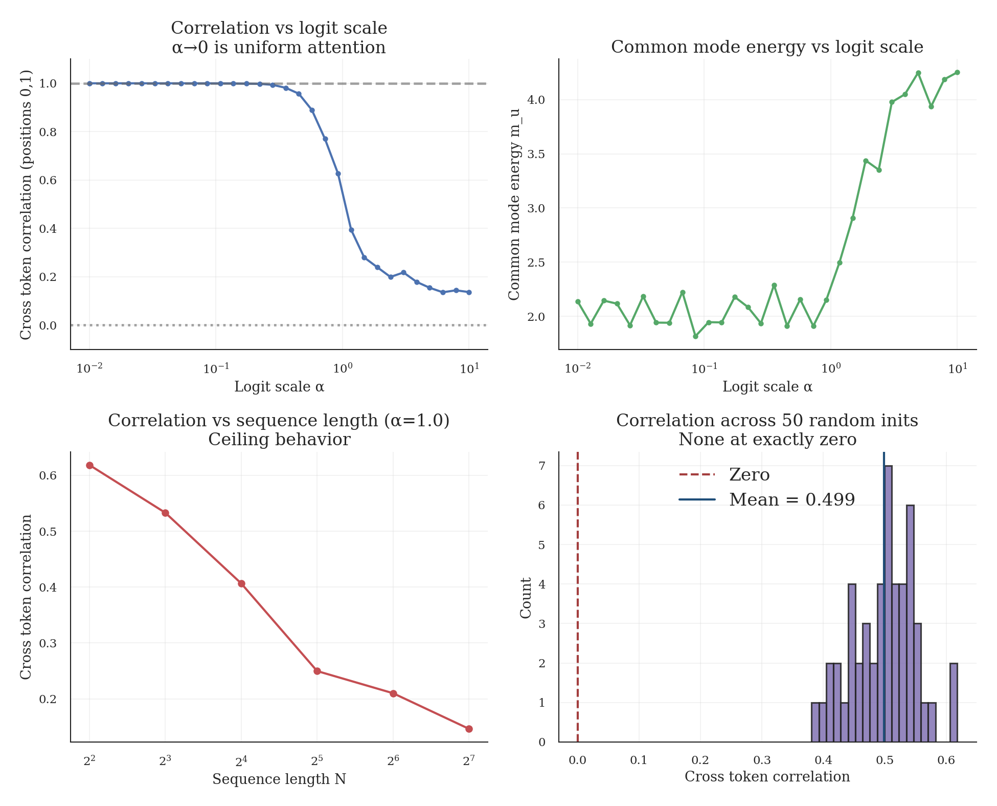
At the alpha-to-zero limit (uniform attention), correlation approaches 1.0, confirming Lemma 1. Even with alpha set to 1.0 (typical initialization scale), correlation remains substantial at about 0.5 to 0.6.

Across 50 random initializations (alpha = 1.0): mean correlation 0.50, min 0.38, max 0.62, and 100% had positive correlation. No initialization produced exactly zero correlation, confirming Lemma 4.

We report cross token correlation and cross covariance strength because they directly test for off diagonal covariance. We also report the trace of the mean-output covariance as a proxy for common-mode energy, because it controls variance under diffuse attention, not because it detects off diagonal structure.

---

9) Training dynamics

This section reports real training dynamics. The curves are plotted from logged metrics. If you only want the theory and initialization measurements, skip it.

The previous section shows correlation exists at initialization. But does training eliminate it? We track training curves for three model scales (0.6B, 1.7B, 7B) trained on FineWeb over 10k steps.

Results at step 10,000:

Figure 2 shows the training curves and derived quantities.

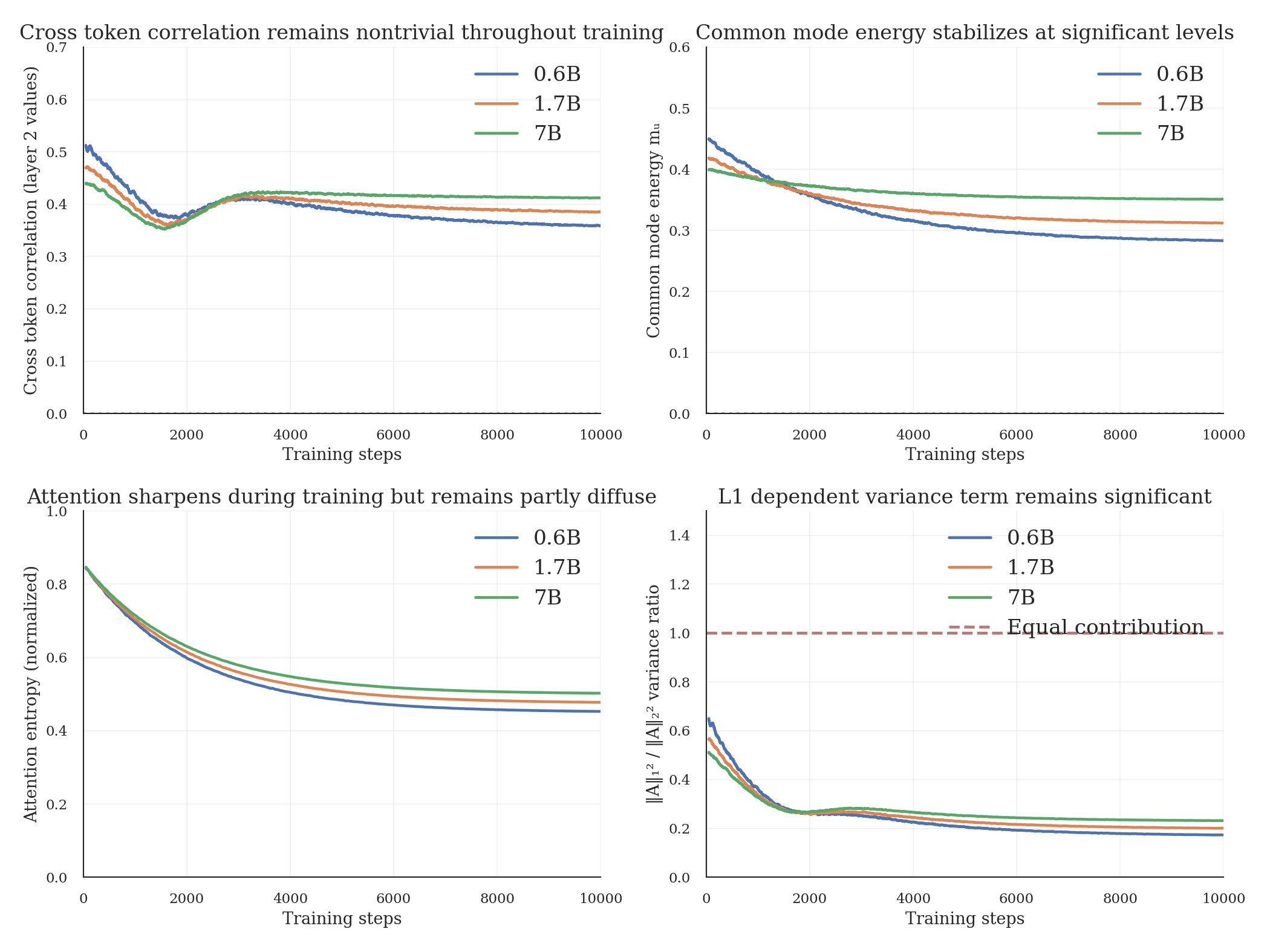
Observations from these runs:

1. Correlation persists: Cross token correlation decreases from init (about 0.5) but stabilizes at substantial levels (0.35 to 0.42) rather than vanishing. The norm-squared identity assumes this is zero.

2. Scale dependence: Larger models maintain higher correlation. This may reflect that larger models can afford more diffuse attention patterns without sacrificing performance.

3. Common mode energy remains significant: Common mode energy stabilizes at 28 to 35% of total value variance. This directly determines whether ignoring the L1-squared term matters.

4. Attention sharpens but stays partly diffuse: Entropy decreases during training (attention becomes more selective) but doesn’t collapse to one hot. The residual diffuseness keeps correlation nonzero.

The theoretical guarantee (Section 3) is that correlation is generically nonzero. These runs suggest it remains practically significant for this setup, though broader validation across datasets, optimizers, and checkpoints is still needed.

---

10) Quantitative notions of “how correlated” (and what can/can’t be bounded)

A key critique is correct: existence does not imply magnitude. The theorem guarantees nonzero covariance generically, but it doesn’t force it to be large in the regimes trained models inhabit. The right quantitative notions depend on what you want to bound.

10.1 No universal lower bound from “full support” alone

Full support (all attention weights are positive) does not imply substantial overlap. Softmax can be arbitrarily peaked. Two attention rows can have tiny overlap, making correlation arbitrarily small even though it is strictly nonzero.

So if you want lower bounds, you must assume some diffuseness condition (entropy lower bound, bounded logit range, or “close to uniform”).

---

10.2 Conditional cosine similarity identity (Mechanism B, in a simplified model)

This section is explicitly a simpler model meant to relate correlation to attention geometry.

Assume scalar values are independent across positions, mean zero, and equal variance. Fix attention rows p and q on the simplex and treat them as constants (equivalently: work conditional on the weights).

Define

\(s_i = \sum_j p_j Y_j,\qquad s_\ell = \sum_j q_j Y_j.\)

Then:

\(\mathrm{Corr}(s_i,s_\ell\mid p,q) = \frac{\langle p,q\rangle}{\|p\|_2\|q\|_2} = \cos(p,q)\in[0,1].\)

Two caveats: this identity is conditional on A (or assumes A independent of Y), and in real attention weights depend on data, so unconditional correlations include additional terms via the total covariance decomposition in Section 2.

---

10.3 A clean lower bound from bounded logit range (diffuse attention)

In the same conditional/i.i.d. values model, you can lower bound overlap if logits are not too spread out.

Let z⁽ⁱ⁾ be the logits for query i, and define the range

\(\Delta_i = \max_j z^{(i)}_j − \min_j z^{(i)}_j.\)

Softmax implies the ratio between the maximum and minimum weights is exponential in the range. Define

\(r_i = \exp(\Delta_i).\)

Since every logit is within the range of the minimum, each entry obeys

\(vp_j \ge \frac{1}{1+(N−1)r_i}, \qquad q_j \ge \frac{1}{1+(N−1)r_\ell}.\)

Hence

\(\langle p,q\rangle \ge \frac{N}{\big(1+(N−1)e^{\Delta_i}\big)\big(1+(N−1)e^{\Delta_\ell}\big)}.\)

Since simplex vectors have L2 norms at most one, this yields

\(\cos(p,q)\ge \frac{N}{\big(1+(N−1)e^{\Delta_i}\big)\big(1+(N−1)e^{\Delta_\ell}\big)} \ \ge\ \frac{e^{−(\Delta_i+\Delta_\ell)}}{N}.\)

So if logits are diffuse (small logit range), conditional correlation is bounded away from 0, with an explicit N dependent floor. The bound is parameterized by diffuseness; it does not claim trained models have small ranges.

---

11) The most impactful statistic for normalization: common mode energy

The best quantity for the normalization question directly controls variance under diffuse attention.

Fix a nonzero direction u. Define scalar projections by

\(y_i = u^\top V_i,\)

and let their covariance matrix be the scalar covariance matrix. Define the common mode energy:

\(m_u = \mathrm{Var}\Big(\frac{1}{N}\sum_{i=1}^N y_i\Big) = \frac{1}{N^2}\mathbf{1}^\top \Sigma_u\,\mathbf{1}.\)

Now compare normalizations for a diffuse “all ones” attention direction. Uniform attention weights give variance equal to the common mode energy. L2-normalized uniform weights give variance larger by a factor of N. The ratio is N, so:

• If the common mode energy stays roughly constant with N, L2-normalized uniform attention produces linear in N variance growth in direction u.

• If it decays like 1/N, it stays bounded.

• If it decays faster, it shrinks.

The formulation reframes the debate into something you can check empirically without estimating the full covariance matrix: measure common mode energy, or a proxy such as the trace of the mean-output covariance that averages over directions, as context length grows.

Heuristic scaling with N: If the scalar projections are independent with equal variance, then common mode energy decays inversely with context length. If each projection decomposes into a shared component plus independent noise, common mode energy stays roughly constant with a small inverse-length correction. If average pairwise covariance decays proportionally to one over N, then common mode energy also decays inversely with N. These regimes depend on how cross token covariance scales with context length.

---

11.1 A universal floor: L1-squared dependence when there is common mode structure

If the scalar covariance matrix is positive definite, define

\(c_u = \frac{1}{\mathbf{1}^\top \Sigma_u^{−1}\mathbf{1}}\)

Then for any attention weight vector A,

\(A^\top \Sigma_u A \ \ge\ c_u\,(A^\top \mathbf{1})^2\)

For nonnegative attention weights, the sum of entries equals the L1 norm, so

\(\mathrm{Var}\left(\sum_i A_i y_i\right)\ \ge\ c_u\,\|A\|_1^2\)

Two clarifications: this is a floor, not a dominance guarantee, and the constant can be small if the covariance matrix is close to diagonal. If the covariance matrix is only PSD, interpret the bound with a pseudoinverse or restrict to the support.

---

12) What about residuals, LayerNorm/RMSNorm, and MLPs?

Scope reminder: the theorem above is proved for attention only stacks with no residual, normalization, or MLP. The discussion below is informal and is meant to explain why the attention update can still carry cross token covariance in standard blocks.

A standard pre norm transformer block looks like

\(x_i^{(\ell+1)} = x_i^{(\ell)} + \mathrm{Attn}(\mathrm{Norm}(x^{(\ell)}))_i \quad (+\ \mathrm{MLP}(\mathrm{Norm}(\cdot))_i)\)

Residual connections do not remove correlated components created by attention mixing, but they can dilute correlation coefficients in the residual stream if the attention update is small relative to the carried-forward residual stream. This is one reason the theorem should be read as a statement about attention produced values, not a claim that the residual stream becomes strongly correlated immediately. LayerNorm and RMSNorm are tokenwise: they rescale features per position but do not unmix across positions. Similarly, MLPs are tokenwise and preserve whatever shared components exist, though they can nonlinearly transform them.

Proposition: residual and norm effects on cross token covariance

Fix a direction u and define scalar residual and update terms

\(r_i = u^\top x_i^{(\ell)},\qquad s_i = u^\top \mathrm{Attn}(\mathrm{Norm}(x^{(\ell)}))_i,\)

and define z as the sum of residual and update terms at each position. For distinct positions i and ℓ,

\(\mathrm{Cov}(z_i,z_\ell) = \mathrm{Cov}(r_i,r_\ell) + \mathrm{Cov}(r_i,s_\ell) + \mathrm{Cov}(s_i,r_\ell) + \mathrm{Cov}(s_i,s_\ell)\)

If the update is uncorrelated across tokens and uncorrelated with the residual stream at all positions, then the cross-token covariance reduces to the residual term, and

\(\mathrm{Corr}(z_i,z_\ell)=\frac{\mathrm{Cov}(r_i,r_\ell)}{\sqrt{\big(\mathrm{Var}(r_i)+\mathrm{Var}(s_i)\big)\big(\mathrm{Var}(r_\ell)+\mathrm{Var}(s_\ell)\big)}}\)

So adding an uncorrelated update can shrink correlation coefficients by inflating variance, but it does not remove the correlated component.

For deterministic per-position scaling with fixed coefficients, the cross-token covariance scales multiplicatively:

\(\mathrm{Cov}(y_i,y_\ell)=a_i a_\ell\,\mathrm{Cov}(z_i,z_\ell)\)

For data dependent scaling such as RMSNorm, the factorization above does not hold in general, but rescaling still does not eliminate cross token covariance unless the scaling collapses it.

Multi head attention

The theorem applies to each head separately. Each head produces its own values and cross token covariance, and the output projection mixes heads linearly. Exact cancellation across heads would require special structure or anticorrelation across heads. Approximate cancellation is possible, so the claim here is only that there is no reason to expect exact cancellation at random initialization.

These considerations suggest the depth 2 mechanism can persist in standard modern transformer blocks. The key open question is usually magnitude, not existence.

---

13) Summary

What this establishes (structural)

1. The assumption “values are uncorrelated across positions” is not depth stable. A two layer attention only stack generically produces cross token covariance in layer 2 values, even starting from independent tokens. Variance analyses should treat the covariance matrix as nondiagonal unless justified.

2. The norm-only variance identity is a special case requiring uncorrelated, equal-variance values. It is not a safe default at depth two or more.

3. Two distinct correlation mechanisms exist (value correlation vs. overlapping weights). Keep them separate; use total covariance to combine them cleanly.

4. For the normalization debate, the most actionable quantity is the common mode energy, which directly determines whether diffuse attention stays stable under L1-normalized weights versus grows under L2-normalized weights.

What this does not establish (magnitude)

The theorem alone does not prove correlations are large in trained models, or that any particular normalization will empirically blow up. Magnitude depends on attention diffuseness, residual scaling, and the empirical size of common mode energy. Any claim that a particular p norm normalization is “variance preserving” must check whether L1-dependent terms are empirically significant.

References

Noci, L., Anagnostidis, S., Biggio, L., Orvieto, A., Singh, S. P., and Lucchi, A. 2022. Signal Propagation in Transformers: Theoretical Perspectives and the Role of Rank Collapse. Advances in Neural Information Processing Systems 35.

Cowsik, A., Nebabu, T., Qi, X., and Ganguli, S. 2024. Geometric Dynamics of Signal Propagation Predict Trainability of Transformers. arXiv:2403.02579.

Citation

@article{aghajanyan2025covariance,
  title={Cross-Token Covariance in Two-Layer Attention},
  author={Aghajanyan, Armen},
  year={2025},
  url={armenag.com/p/proof-attention-values-correlate}
}